prometheus
PromQL Cheat Sheet
https://promlabs.com/promql-cheat-sheet/
Fundamentals
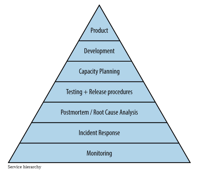
Health of a Service
The health of a Service can be characterized in the same way as the human needs by Maslow:
Metrics
Gauges
Gauges are numbers that go up or down like CPU utilization or number of customers
Counters
Counters are numbers that increase over time and never decrease like number ob bytes sent by a network device or the number of logins.
Histograms
A Historgram is a (graphical) frequency distribution (Häufigkeitsverteilung) of a dataset. The first step is to bucket the range of values and then count observations. The result are multiple metrics: one for each bucket.
Methodologies
The USE Method
This is for host-level monitoring For every resource check
-
Utilization percentage the resource is busy
-
Saturation how much work is queued
-
Errors the count of error events
The Google Four Golden Signals
This is for application monitoring (From the SRE Book)
-
Latency The time taken for a request
-
Traffic requests or transactions per second
-
Errors the rate that requests fail, like HTTP 500
-
Saturation the “fullness” of the applications resources like memory or IO.
Architecture
A Source of metrics that is scraped is called an endpoint. To scrape an endpoint a configuration called target is needed. A group of targets is called a job e.g. a cluster of apache servers.
Data Model
Labels
A time series is identified by its name and labels. But the name is also a label called __name__
There are instrumentation labels which are added at the source before scraping and target labels which are added by Prometheus during and after the scrape.
There are two types of target relabeling: relabel_configs happens before the scrape and metric_relabel_configs happens after the scrape.
Samples
A value in a time series is called a sample. It consists of:
- A float64 value
- A millisecond-precision timestamp
PromQL
CPU utilization percent
100 - avg(irate(node_cpu_seconds_total{job="node",mode="idle"}[5m])) by (instance) * 100
Is load 2 times greater than number of cpus ?
node_load1 > on (instance) 2 * count by (instance) (node_cpu_seconds_total{mode="idle"})
Memory percent used
(node_memory_MemTotal_bytes - (node_memory_MemFree_bytes + node_memory_Cached_bytes + node_memory_Buffers_bytes)) / node_memory_MemTotal_bytes * 100
Rate of paging in and out of memory
1024 * sum by (instance) ( rate(node_vmstat_pgpgin[1m]) + rate(node_vmstat_pgpgout[1m]))
Disk usage percent
(node_filesystem_size_bytes{mountpoint="/"} - node_filesystem_free_bytes{mountpoint="/"} ) / node_filesystem_size_bytes{mountpoint="/"} * 100
Predict linear
predict_linear(node_filesystem_free_bytes{mountpoint="/"}[1h], 4*3600)
Vector match
node_systemd_unit_state{name="docker.service"} == 1 and on (instance, job) metadata{datacenter="NJ"}
Instrumentation
Summary
In order to track request rate and latency a Summary metric is used which creates the two time series sum and count.
Request rate:
rate(request_processing_seconds_count[1m])
Latency:
rate(request_processing_seconds_sum[1m]) / rate(request_processing_seconds_count[1m])
While the summary provides total request_count and latency_sum, it also calculates configurable quantiles over a sliding time window. This is called client-side percentiles. These provide some level of insight but are non-aggregable across dimensions.
Histogram
A histogram with a base metric name of <basename> exposes multiple time series during a scrape:
-
cumulative counters for the observation buckets, exposed as
<basename>_bucket{le="<upper inclusive bound>"} -
the total_sum of all observed values, exposed as
<basename>_sum -
the count of events that have been observed, exposed as
<basename>_count(identical to<basename>_bucket{le="+Inf"})
If your service runs replicated with a number of instances, you will collect request durations from every single one of them, and then you want to aggregate everything into an overall 95th percentile. However, aggregating the precomputed quantiles from a summary rarely makes sense. In this particular case, averaging the quantiles yields statistically nonsensical values:
avg(http_request_duration_seconds{quantile="0.95"}) // BAD!
Using histograms, the aggregation is perfectly possible with the histogram_quantile() function.
histogram_quantile( 0.95, sum(rate(http_server_requests_seconds_bucket{status="200"}[5m])) by (container_name, uri, le)) // GOOD.